Prepare data
Prior to drawing circos plot, you should prepare or import data for plotting. Circhart has five data types including karyotype (band) data, plot data, link data, loci data, text data. Each data type has different columns. The columns are generally separated by a white space.
Karyotype Data
The karyotype data defines the chromosomes and cytogenetic bands. It has seven columns: type, parent, name, label, start, end, color. The name column is an unique id for each chromosome or band. The name is very important, as the other data types must use this name to distinguish different chromosomes.
Column |
Description |
|---|---|
type |
chr (for karyotype) or band (for band data) |
parent |
- (for karyotype) or chromosome name (for band data) |
name |
chromosome uniq id |
label |
chromosome or band label |
start |
start position |
end |
end position |
color |
color name |
The karyotype data example:
chr - hs1 NC_060925.1 0 248387328 chr1
chr - hs2 NC_060926.1 0 242696752 chr2
chr - hs3 NC_060927.1 0 201105948 chr3
...
Note
Karyotype data is essential for creating circos plots. You must prepare or import karyotype data before drawing circos plots.
Import Karyotype Data
If you already have karyotype data, you can import data directly into Circhart. Go to File menu -> Import Data -> Import Karyotype Data, select a file to import karyotype data.
Note
The imported or prepared karyotype data will be assigned data type of karyotype.
Prepare Karyotype Data
If you don’t have karyotype data, you can prepare karyotype data.
Go to Tools menu -> Prepare Data -> Prepare Karyotype Data to open karyotype data preparation dialog:
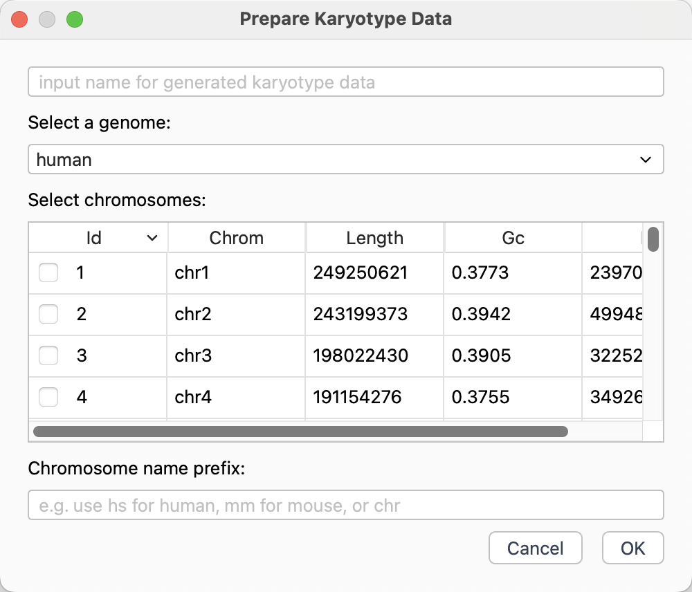
Karyotype data preparation dialog
Input a name for generated karyotype data.
Select a genome and select some chromosomes.
Note
Generally, genome file may have many unplaced sequences that we don’t want to be used for plotting. You can select only the complete chromosomes or chromosomes you desired.
Input an uniq chromosome name prefix. e.g.
hsfor human,mmfor mouse, or you can also simply usechrfor single genome. The circhart will use the this prefix to generate new name for each chromosome. e.g. hs1, hs2, hs3.Click
OKbutton to generate karyotype data based on selected chromosomes.
View Karyotype Data
You can click a karyotype data in Data List to view the karyotype data.
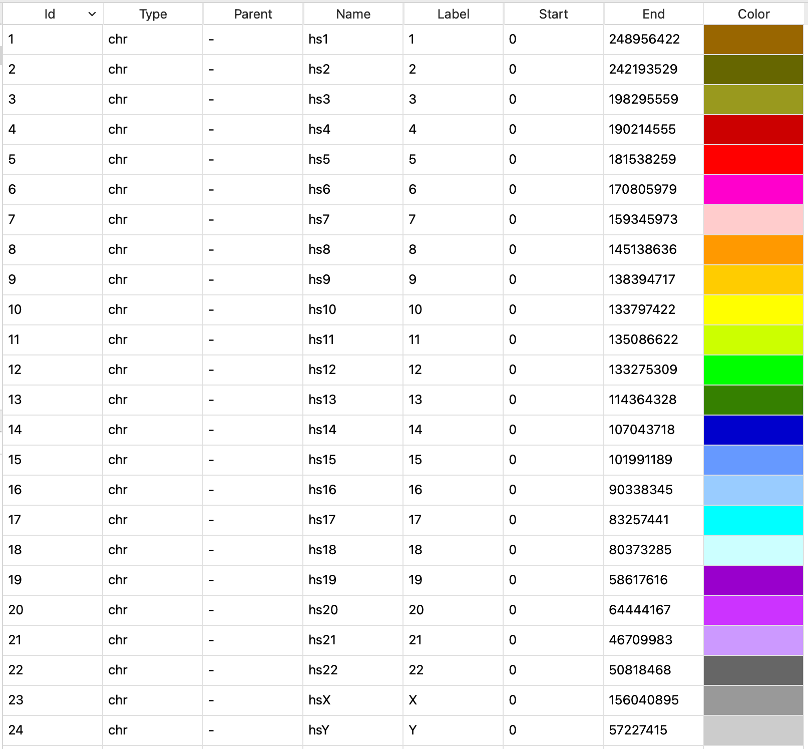
View of karyotype data
Edit Karyotype Data
Circhart allows you to edit the data in columns name and color. Double-click the cell to change name and color.
The karyotype color also can be changed using following methods:
Go to Edit menu -> Karyotype Color -> Set to Default to change colors to default colors.
Go to Edit menu -> Karyotype Color -> Set to Random to change colors to random colors.
Go to Edit menu -> Karyotype Color -> Set to Single to change all colors to a single color.
Band Data
The band data has the same data format with karyotype data. The band data was generally put into karyotype file. Circhart also allows you to import or prepare band data separately.
The band data example:
band hs1 p36.33 p36.33 0 1735965 gneg
band hs1 p36.32 p36.32 1735965 4816989 gpos25
band hs1 p36.31 p36.31 4816989 6629068 gneg
band hs1 p36.23 p36.23 6629068 8634052 gpos25
band hs1 p36.22 p36.22 8634052 12044143 gneg
...
Import Band Data
If you already have band data, you can import data directly into Circhart. Go to File menu -> Import Data -> Import Band Data, select a file to import band data.
Note
The imported or prepared band data will be assigned data type of banddata.
Prepare Band Data
If you don’t have band data, you can prepare band data. Before preparing band data, you should get genome cytobands.
Go to Tools menu -> Prepare Data -> Prepare Band Data to open band data preparation dialog:
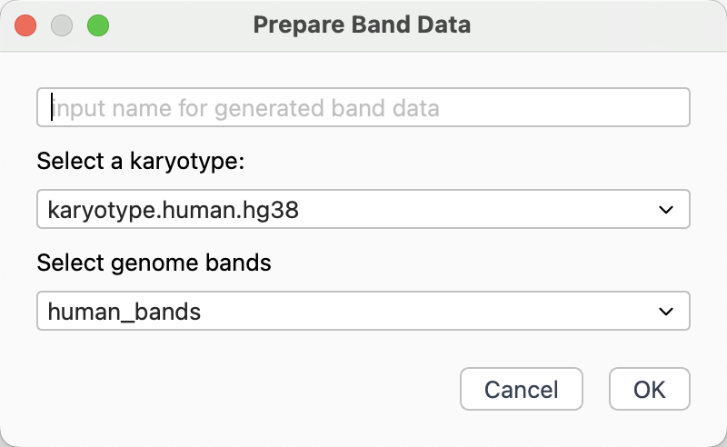
Band data preparation dialog
Input a name for generated band data.
Select a karyotype data.
Select imported genome bands.
Click
OKbutton to generate band data.
Plot Data
The plot data has four required columns (chrom, start, end, value) and on optional column (options). The plot data is used to plot line, scatter, histogram and heatmap tracks.
Column |
Description |
|---|---|
chrom |
chromosome name |
start |
start position |
end |
end position |
value |
integer or decimal |
options |
plot options, usually empty |
Plot data example:
hs1 1000 2000 0.546
hs1 2000 3000 0.423
hs2 4000 6000 0.379
...
Import Plot Data
If you already have plot data, you can import data directly into Circhart. Go to File menu -> Import Data -> Import Plot Data, select a file to import plot data.
Note
The imported or prepared plot data will be assigned data type of plotdata.
Prepare Plot Data
If you don’t have plot data, you can prepare plot data. Circhart can prepare different plot data using different data resource. Circhart supports calculating distribution data using both tumbling window (fixed window without overlap) and sliding window (fixed window with overlap).
Prepare GC Content Plot Data
GC content preparator can help you to calculate GC content within windows.
If no genome data, Go to File menu -> Import Data -> Import Genome File to import a genome.
Go to Tools -> Prepare Data -> Prepare GC Content Data to open GC content preparation dialog.
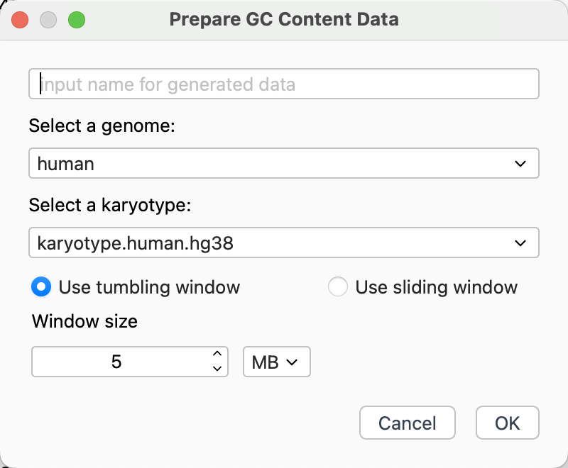
GC content preparation dialog with tumbling window
Input a name for generated GC content data.
Select an imported genome.
Select a karyotype data.
Select tumbling window or sliding window.
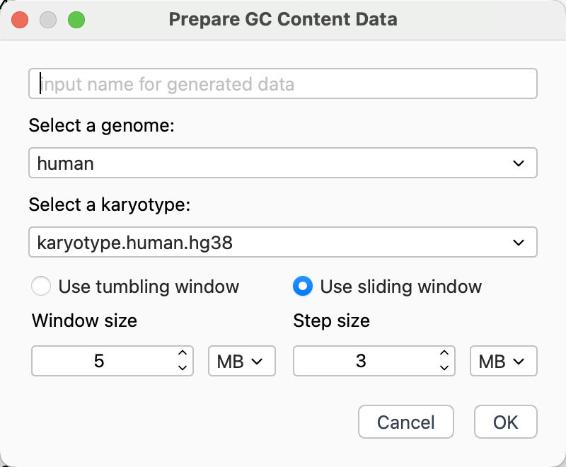
GC content preparation dialog with sliding window
Note
If you select using sliding window, you should also set the step size. Step size should < window size.
Click
OKbutton to generate GC content data.
Prepare GC Skew Plot Data
GC skew preparator can help you to calculate GC skew within windows.
If no genome data, Go to File menu -> Import Data -> Import Genome File to import a genome.
Go to Tools -> Prepare Data -> Prepare GC Skew Data to open GC skew preparation dialog.
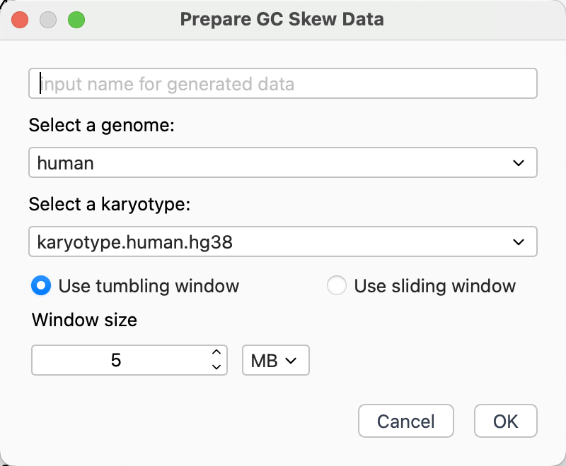
GC skew preparation dialog
Input a name for generated GC skew data.
Select an imported genome.
Select a karyotype data.
Select tumbling window or sliding window.
Click
OKbutton to generate GC skew data.
Prepare Density Plot Data
Density preparator can help you to calculate the number of features from genome annotation file (gtf/gff), the number of variations from vcf file, or the number of regions from bed file winthin windows.
Go to Tools menu -> Prepare Data -> Prepare Density Data to open density preparation dialog.
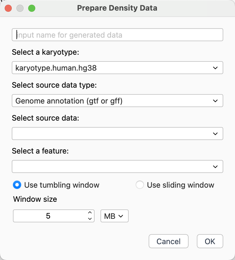
Density data preparation dialog
Input a name for generated plot data.
Select a karyotype
Select source data type according to your imported data.
Select source data.
If Genome annotation (gtf or gff) seleted, you should also select a feature.
Click
OKbutton to generate GC skew data.
Text Data
The text data has the same columns with the plot data. The only difference is that the value column contains text instead of numbers. The text data is used to plot text track.
Text data example:
hs1 144134 146717 SEPTIN14P14
hs1 148562 152332 CICP3
hs1 372945 388041 NOC2L
...
Import Text Data
If you already have text data, you can import data directly into Circhart. Go to File menu -> Import Data -> Import Text Data, select a file to import text data.
Note
The imported or prepared text data will be assigned data type of textdata.
Prepare Text Data
Circhart allows you to extract features as text data from genome annotation file (gtf or gff).
If no annotation data, Go to File menu -> Import Genome Annotation to select a gtf/gff annotation file to import.
Go to Tools menu -> Prepare Data -> Prepare Text Data to open text data preparation dialog.
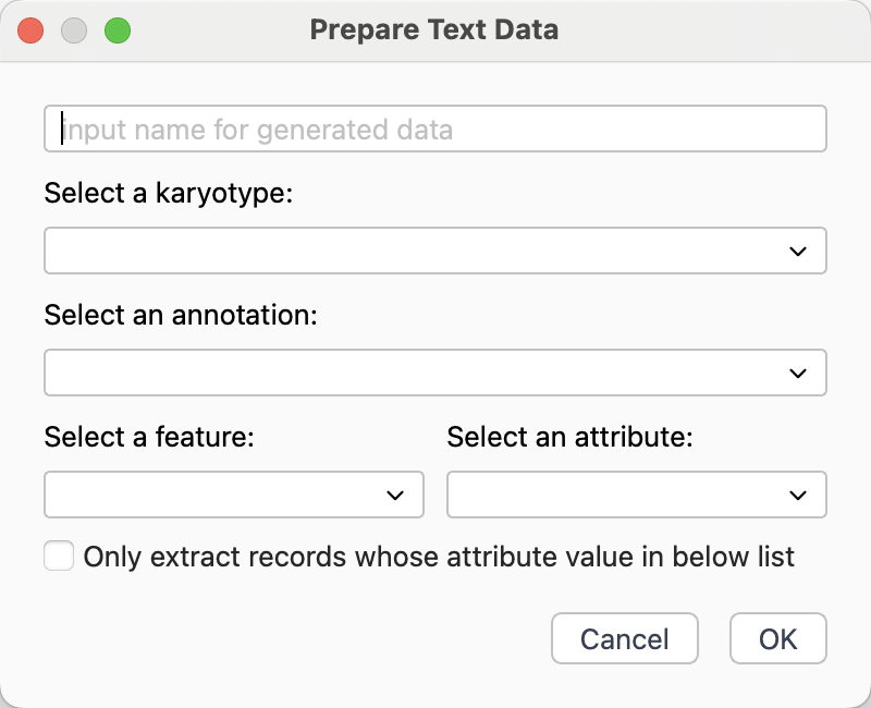
Text data preparation dialog
Input a name for generated text data.
Select a karyotype data.
Select a feature.
Setect an attribute you desired as text value.
Optionally, you can check “Only extract records whose attribute value in below list” to input attribute values (one value per line) to extract matched features.
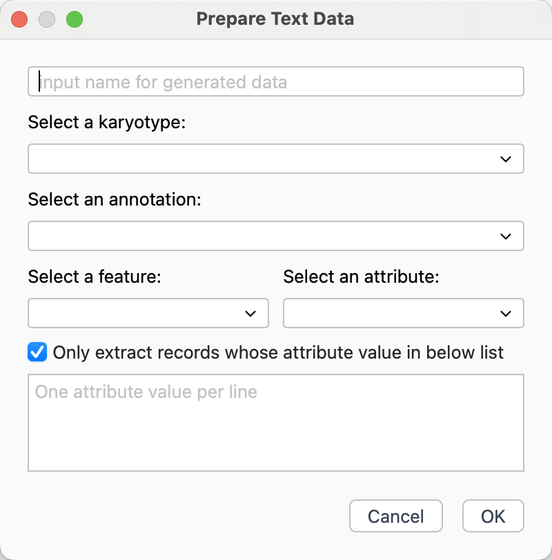
Click
OKbutton to generate text data.
Loci Data
The loci data has three required columns: chrom, start, end and one optional column: options. Each row defines an interval in a chromosome. The loci data used to plot tile, connector and highlight tracks.
Loci data example:
hs1 144134 146717
hs1 148562 152332
hs1 372945 388041
...
Import Loci Data
If you already have loci data, you can import data directly into Circhart. Go to File menu -> Import Data -> Import Loci Data, select a file to import loci data.
Note
The imported or prepared loci data will be assigned data type of locidata.
Link Data
The link data has six required columns: chrom1, start1, end1, chrom2, start2, end2 and one optional column: options. Each row has two intervals on the same or different chromosomes. The link data used to plot link track.
Link data example:
hs1 1000 3000 hs10 2500 3800
hs3 7000 9500 hs8 4000 7000
hs7 500 1500 hs12 5000 6000
...
Import Link Data
If you already have link data, you can import data directly into Circhart. Go to File menu -> Import Data -> Import Link Data, select a file to import link data.
Note
The imported or prepared link data will be assigned data type of linkdata.
Except for above format, circhart also supports importing two-line format file. Links are defined across two lines like:
segdup00001 hs1 465 30596
segdup00001 hs2 114046768 114076456
segdup00002 hs1 486 76975
segdup00002 hs15 100263879 100338121
segdup00003 hs1 486 30596
segdup00003 hs9 844 30515
segdup00004 hs1 486 9707
segdup00004 hsY 57762276 57771573
segdup00005 hs1 486 9707
segdup00005 hsX 154903076 154912373
...
Prepare Link Data
Circhart allows you to prepare link data using the collinearity file generated by MCScanX.
Go to Tools menu -> Prepare Data -> Prepare Link Data to open link data preparation dialog.
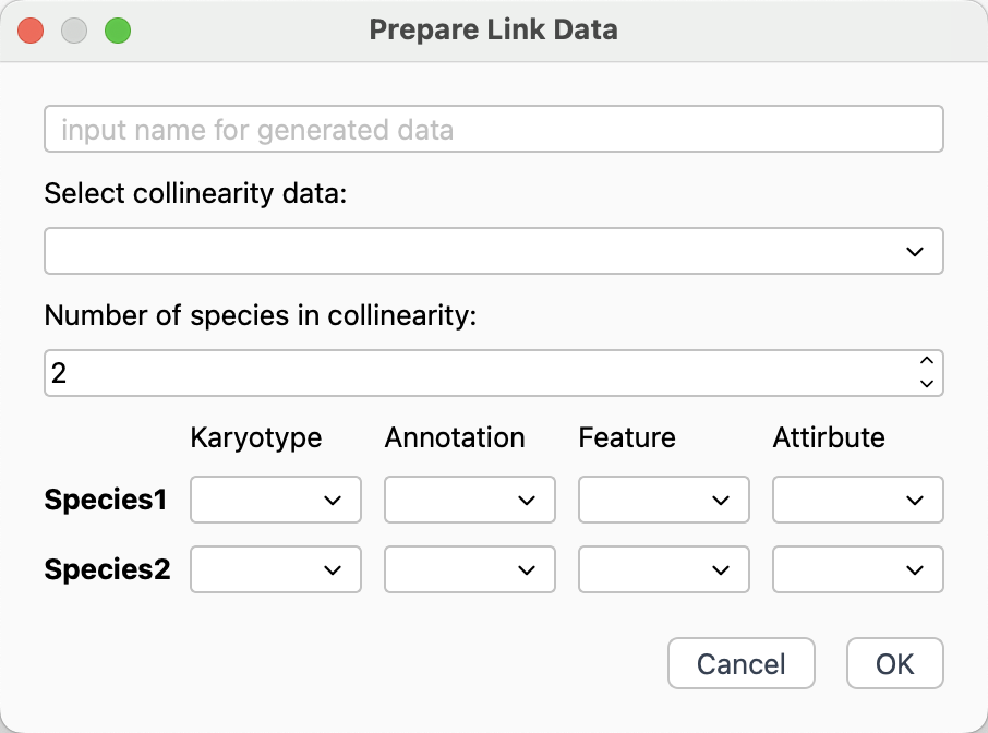
Link data preparation dialog
Input a name for geneated link data.
Select imported collinearity data.
Input the number of species in collinearity data.
Select karyotype and annotation for each species, and select corresponding feature and attribute. Make sure the value of your selected attribute can match the IDs in collinearity file.
Click
OKbutton to generate link data.